Geometry of RREF
Appeal to Reader
If you pay for Medium, or haven’t used your free articles for this month, please consider reading this article there. I post all of my articles here for free so everyone can access them, but I also like beer and Medium is a good way to collect some beer money : ). So please consider buying me a beer by reading this article on Medium.
Introduction
Recently I was asked to create a video demonstrating how reducing a matrix into reduced row echelon form (RREF) uncovers the determinant and looks geometrically. I know this sounds implausible but it happened. So the goal of this post is not to describe all of the properties of a determinant, there are plenty of other resources for that, but to show a nifty demonstration of how the geometry of a matrix is related to the determinant and how by getting a matrix into RREF we uncover the volume of this geometric object. First off, let’s think about how to view a matrix geometrically. Throughout this discussion I will use the matrix:
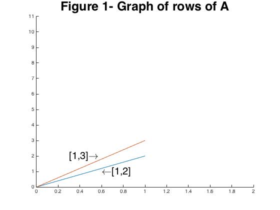
\[A = \begin{bmatrix}1 & 2\\ 1 & 3 \end{bmatrix}\]Visualizing the Matrix
One way to view this matrix is as a collection of row vectors which can be seen in Figure 1.
(This is one of many many ways to do this! I could also think of it as a collection of column vectors for example.) This matrix is also related to the parallelogram in Figure 2 where the absolute value of the determinant is the volume of this parallelogram.
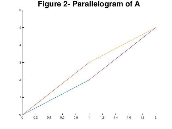
We’ll verify this at the end, but for now just trust me. So taking the determinant \(ad - bc = 1\). That’s great and most of you already knew this but how does performing row reduction on the matrix lead to this? Well as we reduce the matrix we begin to concentrate the values on the diagonal of the matrix. This is basically equivalent to aligning the vectors with the Cartesian axes. To see this let’s make a step in the direction of reduced row form for the matrix \(A\). Let’s take off \(.1 \times A_1\) from \(A_2\) a few times and see what happens.
\begin{align} rref(A) &= \begin{bmatrix} 1 & 2\newline .9 & 2.8\end{bmatrix}\newline &= \begin{bmatrix} 1 & 2\newline .8 & 2.6\end{bmatrix}\newline &= \vdots \newline &= \begin{bmatrix} 1 & 2\newline 0 & 1\end{bmatrix}\newline \end{align}
We can see that we are gradually aligning the bottom vector with the Cartesian axes! If we do the same thing but subtract \(A_2\) from \(A_1\) we will be aligning the other vector. This means that another way of viewing reduced row echelon form is as an axis aligned version of the original matrix. This can be seen in the video below.
Now we can calculate the volume of this parallelogram simply because the height and base sizes are obvious from the diagonal entries they are both 1 and the volume is 1. To verify that the original parallelogram’s volume is 1 we use the standard method of calculating volume and see that: \begin{align} \text{Volume} & =\text{base}\times \text{height} \newline &= ||A_1|| \times ||A_2||\sin \arccos\left(\frac{A_1\cdot A_2}{||A_1||||A_2||} \right)\newline &= \sqrt{5} \times \sqrt{10} \sin \arccos\left(\frac{7}{\sqrt{50}}\right) \newline & = 1 \end{align} Which is indeed 1! Remember that the norm of a vector \(A_1\) can be thought of as a length and that we can find the height using \(\sin (\theta) = \frac{\text{opposite}}{\text{hypotenuse}}\) and \(a\cdot b = ||a||||b|| \cos(\theta)\).