Descent Methods
Overview
Descent methods are a way to solve unconstrained optimization problems which will be the topic of this particular post. In this tutorial we will; talk about some properties of unconstrained optimization problems; solve an example optimization problem using gradient descent with backtracking line search; and solve the same problem with Newton’s method; This post is based on chapter 9 in Steven Boyd and Lieven Vandenberghe’s book Convex Optimization. I have implemented each of the algorithms and methods discussed here in python and they can be found here.
Convexity and Unconstrained Minimization
We are interested in solving the problem \begin{align} \min f(x) \end{align} where f is a convex function and \(f\in \mathcal{C}^2\). If we remember from calculus whenever we want to maximize or minimize a function we find \(x^*\) such that: \begin{align} \nabla f(x^*) = 0\end{align} However this is not always easy to do analytically. So we search for a method which can approximate this optimal solution accurately and quickly. This leads us to a class of algorithms known as descent methods.
Descent Methods
The idea behind the descent methods is to produce a minimizing sequence where \begin{align}x^{(k+1)} & = x^{(k)} + \eta^{(k)}\Delta x^{(k)}\end{align} This is basically saying that at each time step we want to move a small step \(\eta^{(k)}\) in the direction of \(\Delta x\). Here \(k\) denotes our iteration number and \(x\in \mathbb{R}^n\). We are interested in descent methods which are a class of methods such that whenever \(x^k\) is not optimal we have: \begin{align}f(x^{(k+1)}) < f(x^{k})\end{align} Most descent algorithms come in this flavor and the differences arise in how they particular algorithms choose to address the questions, what direction should we move in? How large of a step should we take? When do we stop moving?
Stepsize \(\eta\)
There are a number of ways to determine the stepsize which should be used and there is no perfect answer. The simplest thing to do is choose some small constant and set the stepsize equal to that in machine learning this is known as the learning rate and is most often determined using cross validation. Here we will discuss two slightly better methods for choosing how large of a step to take. The first is known as exact line search. This method chooses \(\eta\) so as to minimize the original function \(f(x)\) along some line segment \(\{x+\eta\Delta x\}\) \(\forall \eta \geq 0\). It should be noted here that this method requires solving an additional optimization problem: \begin{align} \eta = \text{arg}\min_{s \geq 0} f(x + s \Delta x) \end{align}. What this implies is that this method should be used when the cost of computing the search direction \(\Delta x\) is very large. The next method commonly used is known as backtracking line search. This method starts with a stepsize of 1 and gradually reduces it by a factor of \(\beta\) until \(f(x + \eta \Delta x) > f(x) + \alpha \eta \Delta f(x)^T\Delta x\).
Where to Step \(\Delta x\)
Now That we have some methods to find out how big of a step to take we need to figure out in which direction to take that step. The simplest thing to do would be to take a step in the direction of steepest descent. In other words, the direction should be that of the negative gradient. This is exactly what vanilla gradient descent is doing! This algorithm proceeds by:
- set \(\Delta x = -\nabla f(x)\)
- Do some form of line search to choose a step size \(\eta\)
- update our optimal point \(x^{(k+1)} = x^{(k)} + \eta^{(k)}\Delta x^{(k)}\)
- repeat until we are sufficiently close to optimal
To see what this looks like let’s examine gradient descent with backtracking line search on the function \(\frac{1}{2}(x_1^2 + 10x_2^2)\). You can visualize this function as the 3D analogue of a parabola.
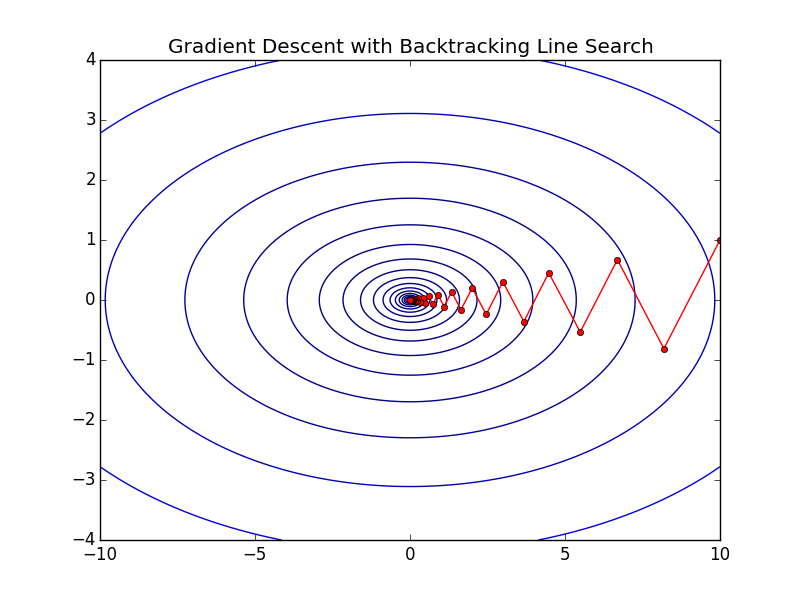
Each red dot represents a different \(x^{(k)}\) and as you can see they pretty quickly zig-zag to the optimal point of this function. The exact number of iterations is 60 in this particular experiment starting at point \(x = [10,1]\). This seems good, and it is, but this is an extremely well behaved function. What happens when the function is a little bit less well behaved. To demonstrate some of the shortcomings of this algorithm we look at it’s performance on a particular instance of the Rosenbrock Function: \begin{align} f(x) = 100(x_2 - x_1^2)^2 + (1 - x_1)^2 \end{align}
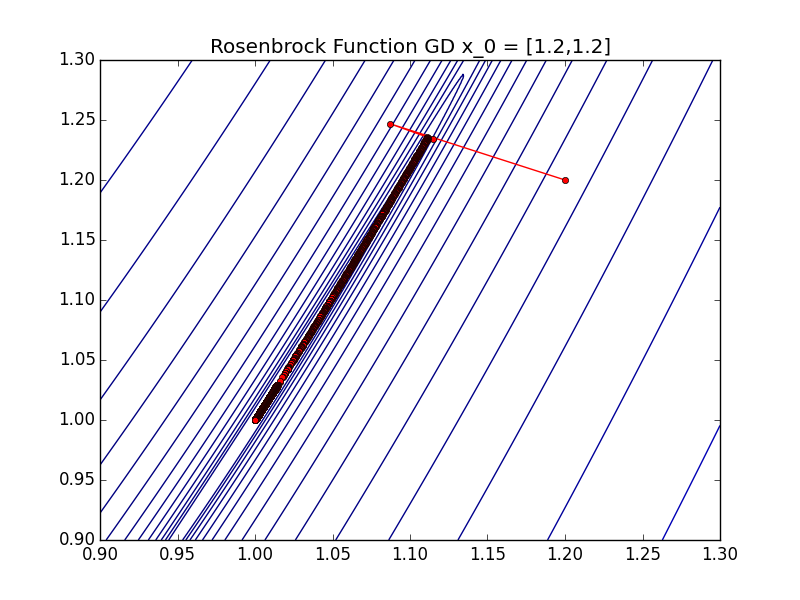
The optimal point of this function is at \(x^* = [1,1]\) Here we start at \(x_0 = [1.2,1.2]\) which is very close to optimal but it takes us 7230 iterations to reach the optimum! This is because the Rosenbrock function has a very steep descent to a large trough which leads to the optimum. As you can see when the direction \(\Delta x\) is very small it can lead to long convergence times. In these instances pure gradient descent does not perform very well. (You can tell if things like this might happen by looking at the condition number of your function I will do a post on convergence and condition numbers at a later date.)
Newton’s Method to the Rescue!
One way to solve this problem is to use additional information about the function. That is exactly the idea behind newton’s method. Here we use second-order information about the function to improve convergence. Namely, we add information about the local concavity of the function in the form of the Hessian of \(f(x)\). This algorithm proceeds as:
- set \(\Delta x = -\nabla^2 f(x)^{-1}\nabla f(x)\)
- find \(\lambda^2 = \nabla f(x)^T\nabla^2 f(x)^{-1}\nabla f(x)\)
- If \(\frac{\lambda^2}{2} \leq \epsilon\) Return
- Do some form of line search to choose a step size \(\eta\)
- update our optimal point \(x^{(k+1)} = x^{(k)} + \eta^{(k)}\Delta x^{(k)}\)
- repeat until (3) returns
Running Newton’s method on the Rosenbrock function is shown below:
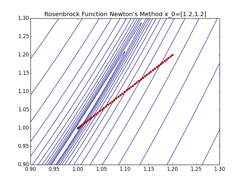
Now it only takes 51 steps to reach the optimal point. With this additional information we can achieve 2 orders of magnitude fewer steps! However it is important to note that this method requires us to compute the Hessian of the function in question, and in many real world applications this is either too expensive or not possible. If this is the case for your particular application you can try a Quasi-Newton method where the Hessian information isn’t computed directly but estimated.