Least Squares and Noise Reduction
Overview
I recently saw a cool way to use Least Squares to reduce noise in a signal and thought that I’d make a post describing it. In this post I will solve a simple optimization for noise reduction in python. paper.
Problem Definition
Imagine that we have some noisy signal \(b_i\) where we assume that our noise is randomly
generated from a standard normal distribution. We want to try and find the true signal
using optimization. To do this we can:
\begin{align}
\min_x ||x-b||^2 + \lambda ||Lx||^2
\end{align}
Where:
\begin{align}
L &= \begin{bmatrix}
1 & -1 & 0 & 0 & \cdots & 0 & 0\newline
0 & 1 & -1 & 0 & \cdots & 0 & 0\newline
0 & 0 & 1 & -1 & \cdots & 0 & 0\newline
\vdots & \vdots & \vdots & \vdots & & \vdots & \vdots\newline
0 & 0 & 0 & 0 & \cdots & 1 & -1
\end{bmatrix}
\end{align}
This basically tries to find \(x\) such that we have the smallest distance between \(x\) (the true signal) and \(b\) (our noisy signal) and the difference between \(x_i\) and \(x_{i+1}\) is small. Our \(L\) matrix just helps us compare two successive \(x_i\)’s. This should also make intuitive sense. I know that my true function should be close to my noisy one so \(||x-b||^2\) should be small. I also know that the signal should not vary wildly from one time point to the next, in other words it should be somewhat smooth \(||Lx||^2\). All that’s left to describe is the role of lambda, which is just a constant that says how much we should focus on making the function smooth. We will explore how lambda affects our noise reduction in the experiments section.
For this experiment I chose my signal to be: \begin{align} b_i &= \sin\left(4\frac{i -1}{299}\right) + \left(4\frac{i -1}{299}\right)\cos^2\left(4\frac{i -1}{299}\right) + \epsilon_i \end{align} Where \(\epsilon_i\) is my noise.
Solving the Problem
To solve this all we really need is Calculus I! We just take the derivative and set it equal to 0. That’s it! \begin{align} f(x) &= ||x-b||^2 + \lambda||Lx||^2\newline &= (x-b)^T(x-b) + \lambda x^TL^TLx\newline &= x^Tx - 2x^Tb + b^Tb + \lambda x^TL^TLx\newline \frac{df}{dx} &= 2x -2b + 2\lambda L^Lx\newline 0 &= 2x -2b + 2\lambda L^TLx\newline b &= (I + \lambda L^TL)x \end{align} And voila! This solution final result looks exactly like a linear least squares problem, luckily we know how to solve Least Squares problems very well so we can find the optimal line super easily. In the next section you will find the code used to do this optimization.
Code
import numpy as np
from matplotlib import pyplot as plt


def gen_signal(samples):
    """Generates the signal described above

    Args:
        samples: (np.array) array of sample points

    Returns:
        sig: Numpy array of the signal with Gaussian noise added
    :return:
    """
    return np.sin(4 * (samples - 1) / 299.0) +
           (4 * (samples - 1) / 299.0) *
    	   np.cos(4 * (samples - 1) / 299.0) ** 2 +
    	   np.random.randn(len(samples)) * .1


def l_mat(n):
    """Generates the L matrix

    Args:
        n: (int) Dimension of L

    Returns:
        (numpy.matrix) of ones and off diagonal -1
    """
    L = np.matrix(np.eye(n - 1, n))
    for i in range(0, n-1):
        L[i, i+1] = -1
    return L

def main():
    samples = np.array(range(0, 300))
    L = l_mat(len(samples))
    signal = gen_signal(samples)
    plt.plot(samples, signal, 'or', ms=2.5)
    for lam in [1, 10, 100, 1000]:
        fit = np.linalg.lstsq(np.eye(L.shape[1], L.shape[1])+lam * np.dot(np.transpose(L), L), signal)[0]
        plt.plot(samples, fit, '-', label='$\lambda =$' + str(lam))
    plt.legend(loc=2)
    plt.show()
Experiments
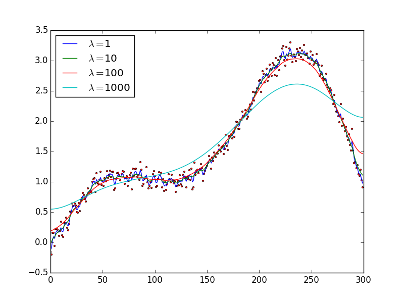
If you run the above code for a few different values of \(\lambda\) you can begin to see how it affects the model. In the figure below, observe how as \(\lambda\) increases it begins to flatten out the curve. Lower values of \(\lambda\) cause us to have spikey fits, that are very close to the original noisy data but are not very smooth. Larger values of \(\lambda\) cause our fit to be too flat penalizing changes in the \(y\) axis more. From the graph below it looks like \(\lambda =10\) is a pretty good fit.