Practical SVD for Data Mining
Introduction
I’ve wanted to discuss how to use the Singular Value Decomposition (SVD) for pattern recognition and data exploration. This is a very powerful technique. Conceptiually you can think of the technique as finding the optimal axes for which you can view your data. Think about the cartesian coordinate system. It is very easy to navigate this space for us simple humans. However, What if your data is skewed and most of it moves along axes which are some rotation of the standard coordinate systm? This is where the SVD can be helpful. It can reveal these optimal basis for your data. In this tutorial I will step through how the SVD can be used to uncover patterns in a synthetic dataset. I’m not going to discuss the mathematics of the SVD in too much detail because there are plenty of other tutorials out there. If you do have questions about the mathematics feel free to email me :).
Traveling Wave
We will use a traveling wave as our example dataset. A traveling wave is a periodic function that moves with constant speed in space and time. For this example we will be examining a 2-D traveling wave. You can visualize this as what a wave moving down a string through time would look like. In python we will generate a simple one using the below function.
def traveling_wave():
    mat = np.matrix(np.zeros([1000, 30]))
    for a in range(0, mat.shape[0]):
        for b in range(0, mat.shape[1]):
           mat[a, b] = np.sin((a / 500.0 - b / 7.5) * math.pi)
    return mat

wave = traveling_wave()
We can think of this data set where each row represents a discrete position on our string, each column represents a discrete point in time, and each element in the matrix is the height of the string at that postition in space and time. Let’s assume that you are given the data found in the variable wave. I visualized this data as a simple raster array as seen in Figure 1.
plt.figure(figsize = (10,10))
ax = sns.heatmap(wave, square=False, xticklabels=False, yticklabels=False, cmap="coolwarm")
plt.xlabel("Time")
plt.ylabel("Spatial position")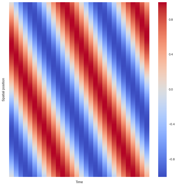
SVD First Steps
Okay now we have some data about the position of the string in space and time. What can we learn about this particular dataset? Some questions that come to mind are:
-
What are the patterns accross space? time?
-
Is this data generated by a single frequency or composed of multiple signals?
Let’s see if we can answer these questions using the SVD. In python performing this decomposition is very simple and can be done in one line of code.
U, S, V = np.linalg.svd(wave, full_matrices=False)This breaks our dataset into three matrices that can be multiplied as \(USV^T\) to recover our original dataset. \(U\) is the left eigen basis \(V\) is the right eigen basis and \(S\) is a diagonal matrix of the singular values. These matrices are constructed such that each column of \(U\) and each Row of \(V^T\) account for as much of the variation in the rows and columns of the data as possible in decreasing order, such that all of the besis elements are orthonormal. This is not a discussion of the mathematics of SVD for an excellent introduction see Gilbert Strang’s video . What is important is that we can interpret the singular values as the importance of the corressponding column in \(U\) and row of \(V^T\) in characterizing the total variation of the dataset. In other words, the first singular value tells me how important the patterns in column 1 of \(U\) and row 1 of \(V^T\) are to describing the dataset. Let’s take a look at those patterns Below I visualize the first three columns of \(U\) and then the first three rows of \(V^T\). What do you notice?
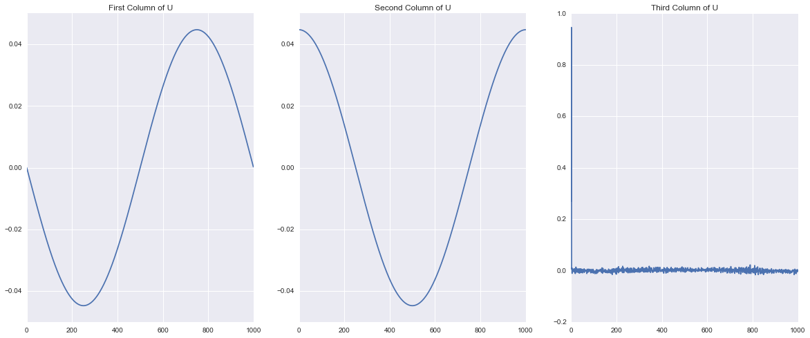
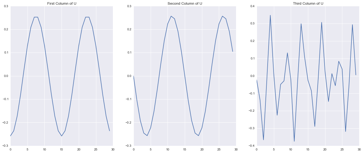
One of the first things that becomes visible is that it looks like the first two patterns are periodic in both \(U\) and \(V\). We can also see that the periodic signals in \(U\) are a single period and those in \(V\) comprise two periods. This makes sense because of our original definition of the traveling wave! In our original wave we made a single period propagate through space but took two periods in time and the SVD uncovered this same structure! This shows how the columns of \(U\) represent patterns that occur accros “space” or the rows of the matrix and the rows of \(V^T\) represent patterns that occur accross “time” or the columns of the matrix.
Do you notice anything strange about the third pattern? It appears to be just a bunch of noise. Now The first two patterns are clearly orderly and the third looks nasty, but I can’t just throw away the third column because it looks bad it might be important to the overall patterns that we are seeing. How can we tell?
Singular Values and Pattern Significance
One of the wonderful things about using the SVD for pattern extraction and data exploration is that it gives us some very useful information about how important each pattern is to characterizing the data in the form of the singular values. Let’s quickly plot the singular values of the data.
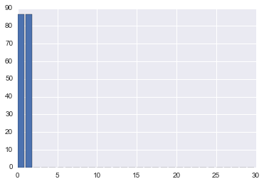
As you can see the first two singular values are very large and the rest are imperceptible. If we look at the first 5 elements wer get:
[ 8.66025404e+01 8.66025404e+01 4.66772947e-14 2.79316542e-14 1.65098443e-14]
One property of the SVD is that we can organize the matrices such that the singular values occur in decreasing order. This means that \(S[0] \geq S[1]\), \(S[1] \geq S[2]\) so on and so forth. From this it is clear that both pattern one and pattern two have equal significance, and pattern three and onward are virtually zero. To conceptually see why this is the case think about what happens when we perform the matrix multiplication \(X=USV^T\) where \(X\) is our original matrix. Each column of \(U\) and each row of \(V^T\) are getting multiplied by the corresponding diagonal element of \(S\). If this number is really big then these rows and columns will contribute more to each element of \(X\).
Let’s turn our attention to that pesky third pattern. As a data scientist we need to make some assumptions when it is appropriate and now is one of those times. Pattern three and beyondfloating point error and I will consider them to be zero. Here it is clear, because this is a contrived example, that there are only two real patterns. So let’s just say that all numbers less than \(1\times 10^{-10}\) are really zero and get rid of them.
S[S <= 1e-10] = 0In a later post I will discuss looking at entropy to quantitatively determine how much of the overall variation is accounted for by any single singular value.