Priors
Introduction
I’ve been playing around a little with parameter estimation and Bayesian statistics and thought that I’d make a quick little visualization of how prior beliefs affect our posterior distribution. In this tutorial we will walk through thinking about whether or not a coin is fair and visualize how our estimate changes with data with respect to our prior beliefs. Let’s get started!
Appeal to Reader
If you pay for Medium, or haven’t used your free articles for this month, please consider reading this article there. I post all of my articles here for free so everyone can access them, but I also like beer and Medium is a good way to collect some beer money : ). So please consider buying me a beer by reading this article on Medium.
Problem
You’re in Vegas watching people bet on the outcome of a coin toss. If it is heads then you win double your bet and if it is tails the house takes your money. You decide to count the number of times that you see each outcome and want to determine the value of the coin. Let \(H\) be the probability of getting heads using the Casino’s coin, and let \(D\) be the data set of our tosses. Let’s assume that we saw 100 coin tosses and out of those 100 tosses 40 of them were heads. What is the weighting of the coin? Naturally you would say that \(H=\frac{40}{100} = .4\) but how did you get that number? Let’s walk through the derivation!
Maximum Likelihood Estimation
We are estimating a coin toss which means that our data will take on one of two values with probabilities \(p\) and \(1-p\). Thus we will assume that our data is generated by a Bernoulli distribution, or in other words the likelihood of the data given a particular probability of heads is \(P(D | H) \propto H^k(1 - H)^{n-k}\). Now we want to figure out what value of \(H\) maximizes this likelihood function. Since the natural logarithm will not affect our maximum we can solve for the maximum of the log instead. It will make the math easier trust me.
\begin{align} \log P(D | H) &= \log(H^k(1 - H)^{n-k}) \newline &= k\log(H) + (n-k)\log(1-H) \end{align}
Now refer back to your good ol’ Caclulus I class, take a derivative and set it equal to 0 in order to identify the critical points.
\begin{align} \frac{dP}{dH} &= \frac{k}{H} - \frac{n-k}{1-H} \newline 0 &= \frac{k}{H} - \frac{n-k}{1-H} \newline nH-kH &=k-kH\newline H &= \frac{k}{n} \end{align}
It appears that our intuition was correct, and the best estimate for the probability of heads is the number of heads tossed out of the total number of tosses.
Priors
However there is some potential hidden information here that we didn’t address. We are gambling in Las Vegas after all, and maybe the casinos are a little shady. In our model we assumed that the parameter \(H\) could take any value between 0 and 1 with equal probability. This assumption about what values our parameters can take is called a prior and for this analysis we assumed a uniform prior.
\begin{align} P(H) &= \begin{cases} 1, 0 \leq H \leq 1\newline 0, \text{otherwise}\newline \end{cases} \end{align}
This particular prior says that we have absolutely no information about what the probability of heads should look like. It is a good assumption if we don’t know anything about our parameters, but in the case of a common quarter this might be a bad assumption because we know that common street coins are very close to fair. The prior is combined with the likelihood to generate the posterior distribution using Baye’s rule.
\begin{align} P(H|D) &\propto P(D|H)P(H) \end{align}
These priors have an important affect on our model when the sample size is small and their effect diminishes as the sample gets larger. Let’s see this effect in action for a few different priors.
We already know what our posterior looks like for a uniform prior but what about if we assume that the casino is playing by the rules and using a common street coin. Then we might assume a gaussian prior with mean .5 and a small standard deviation. Then our posterior distribution would be:
\begin{align} P(H|D) &= {n\choose k}H^k(1 - H)^{n-k} \frac{1}{\sigma\sqrt{2\pi}}e^{-\frac{(H-\mu)^2}{2\sigma^2}} \end{align}
For this implementation I chose a mean of \(.5\) because fair coins should be close to even and a standard deviation of \(.05\) so that if the coin happens to be unfair it is going to sit between .4 and .6.
Lets take a look at one more possible prior where we think that there might be a high likelihood that the coin is extremely biased. In this case we could use the beta distribution which would make our posterior:
\begin{align} P(H|D) &= {n\choose k}H^k(1 - H)^{n-k} \frac{\Gamma(\alpha+\beta)}{\Gamma(\alpha)\Gamma(\beta)}H^{\alpha-1}(1-H)^{\beta-1} \end{align}
The pdf of this function for \(\alpha=.1,\beta=.1\) is:
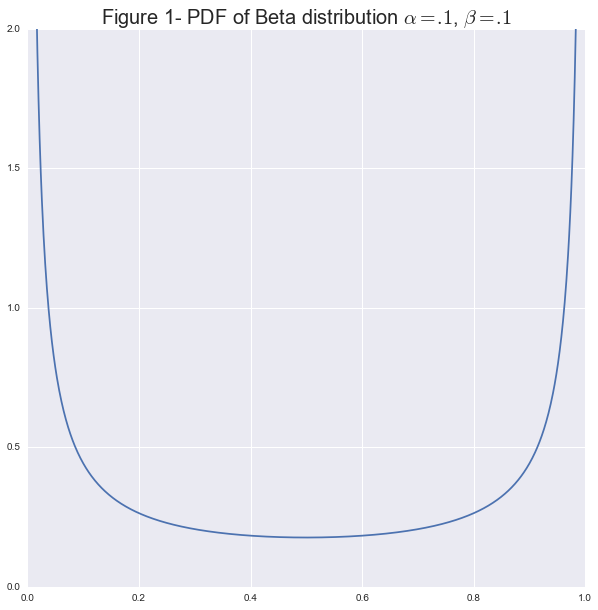
Notice how most of the probability is concentrated at the extremes. This fits with the idea that the coin is very likely to throw all Heads or all Tails.
We can generate these posteriors in python using the following functions:
def posterior_uniform_prior(H, k, n):
    return scipy.special.comb(n,k) * H**k * (1 - H)**(n - k)

def posterior_gaussian_prior(H, k, n, std=.05, mu=.5):
    return scipy.special.comb(n,k) * H**k * (1 - H)**(n - k) * 1 / (std * math.sqrt(2 * math.pi)) * np.exp(-(x - mu)**2 / (2 * std**2))

def posterior_beta_prior(H, k, n, a=.1, b=.1):
    normalizer = scipy.special.gamma(a + b) / (scipy.special.gamma(a) * scipy.special.gamma(b))

    return scipy.special.comb(n,k) * H**k * (1 - H)**(n - k) * normalizer * H**(a - 1) * (1 - H)**(b - 1)

def beta(x, a, b):
    normalizer = scipy.special.gamma(a + b) / (scipy.special.gamma(a) * scipy.special.gamma(b))
    print normalizer
    return normalizer * x**(a - 1) * (1 - x)**(b - 1)
Now let’s look at how the priors affect our parameter estimation visually. First let’s generate a set of coin flip experiments for \(H=.3\)
# Number of flips in each trial
n_vals = [0, 1, 2, 3, 4, 5, 16, 32, 64, 128, 256, 512]

# Simulate the number of heads drawn from a coin with H=.3
k_vals = []
H = .3
for n in n_vals:
    k_vals.append(np.sum(np.random.binomial(1, H, n) == 1))
Below I have plotted the evolution of the posterior with increasing evidence (Larger number of flips observed) let’s take a look and see what we can learn.
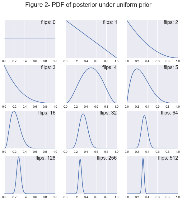
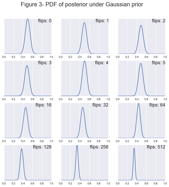
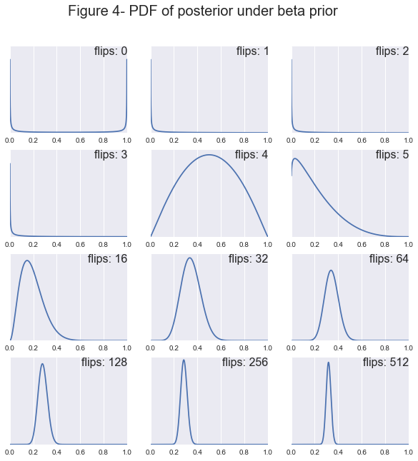
First off notice how as the sample size increases all of the posteriors tend toward a normal distribution centered at \(H=.3\). You can see clearly that the prior has a large effect when the sample size is small and as the sample size increases the likelihood begins to dominate. Also notice how the prior can affect the convergence rate of the posterior. For example, for both the uniform and beta prior after 64 flips the coins true bias falls within our 95% confidence interval, whereas for the Gaussian our true bias doesn’t appear in our interval until around 256 flips. The takeaway message here is that if we start out not knowing much about our value, uniform or beta distribution it is easy to convince the model that the coin is biased. Whereas, if our model has a strong belief that the coin is fair, i.e. the Gaussian prior, then it will take much more data to convince it that the coin is in fact not fair.