Facial Recognition and Machine Learning Advice
Introduction
One of my favorite lectures I attended while learning about machine learning was on practical advice for building machine learning systems. I felt like over the course of the semester I had learned a lot about different algorithms and applications but what to do after the simple classifier was build remained a mystery. This lecture shed a bit of light on this question of how to further improve an ML system after it’s already built and I’d like to use this post to go from the beginning to end and build a solid machine learning application. The example problem that we will takle here is that of facial recognition. Given an unknown persons face, and a set of training faces can we identify the unknown individual. I will assume that the unknown individual we are identifying has been seen by our classifier. Alright let’s get started.
Basic System
Before I begin any ML system I like to think of the problem in terms of Tom Mitchell’s definition of machine learning. Which is:
“A computer program is said to learn from experience E with respect to some class of tasks T and performance measure P if tis performance at tasks in T, as measured by P, improves with experience E.”
This lends itself nicely to deconstructing the problem into three pieces the experience, or data that the system will use to learn, the task, which in this case is recognizing an individuals face, and the performance measure or how the system will be judged which in this case we will talk about precision.
Now that we have the basic components of our system we can start to think about how to approach the problem. The first question is what data are we going to use to train our learner? Since we are trying to recognize faces we’ll need some data set of people’s faces to learn from. I chose to use the Yale face data set. You can find the data set here.
With the data in hand we can begin to think about our task and how to use the data to solve it. Each of the images in the Yale face data set is \(243 \times 320\) pixels. The next question which naturally arises is how do we turn these raw pixels into something meaningful in order to help the computer learn? There are many ways to do this. We could use the raw pixels as our features but the problem here is that then we are left with 77,760 features and most of them are probably not very useful. Think about the edges of the croped image. For most of the pictures these regions contain almost no information. If we were to use raw pixels we’d be including the noise in these regions into our model. This is definitely not ideal. The next thing we can try is extracting more meaningful features from this data. To do that we will use PCA.
Featurizing Faces
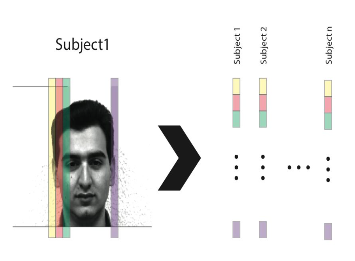
The intuition behind using PCA is that we have a very high dimensional space (77,760) but we believe that in order to describe a face we don’t need all 77,760 dimensions. Through PCA, we can find a lower dimensional subspace that will characterize human faces well. To begin we need to vectorize each face by unfolding it columnwise and concatenate them into a matrix as seen below.
def find_label(name):
    """
    This method extracts the label of the individual in the yale face data set.

    Args:
        :param name: (string) The file name for which we want to extract the face label

    Returns:
        :return: (Int) the integer label of the subject in the yale face data set
    """
    return int(name.split(".")[0].split("t")[1])

# Import data
directory = "../Data/yalefaces"
files = os.listdir(directory)

# Create Label vector
labels = []
for file in files:
    if not file == ".DS_Store":  # I'm on a Mac so I need to ignore this file
        labels.append(find_label(file))

labels = np.array(labels)

# pull the first image to initialize the matrix
img = misc.imread(directory + "/" + files[1])
del files[1]
faces = np.matrix(img.flatten("F")).T

# load in all images, vectorize them, and compile into a matrix
for file in files:
    if not file == ".DS_Store":
        img = misc.imread(directory + "/" + file)
        faces = np.concatenate([faces, np.matrix(img.flatten("F")).T], axis=1)
Now we want to center the data based on the average face by subtracting off the mean face from each column. We will refer to vectorized face \(i\) in the data set as \(\Gamma_i\), and the average face as:
\[\Psi = \frac{1}{n}\sum_{i=1}^n\Gamma_1\]This will help reduce some of the effects of lighting and slight individual movement. The mean face \(\Psi\) can be seen below.
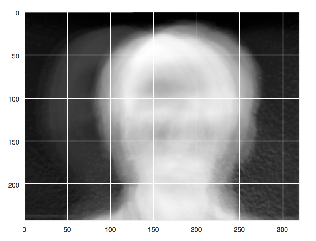
Notice how it appears face like, yet there are some airy boundaries around where the head appears. This is because most of the faces are pretty close to center but some vary a bit in their positioning. Subtracting this mean face off helps us account for some of this variation.
On to the fun part, learning. We can decompose our face matrix as:
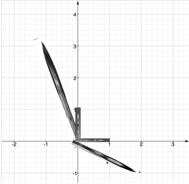
\[A = U\Lambda U^T\]We can think of each column of \(U\) as a principle axis in the subspace of faces. Let’s explore this further. Imagine that we have a 77,760 dimensional space and each face is represented by a vector in this space. We want to find the subspace that that is primarily inhabited by human faces. This is kind of like if face space happened to be a plane then we could represent it by two independent vectors \(u\) and \(v\) like so.
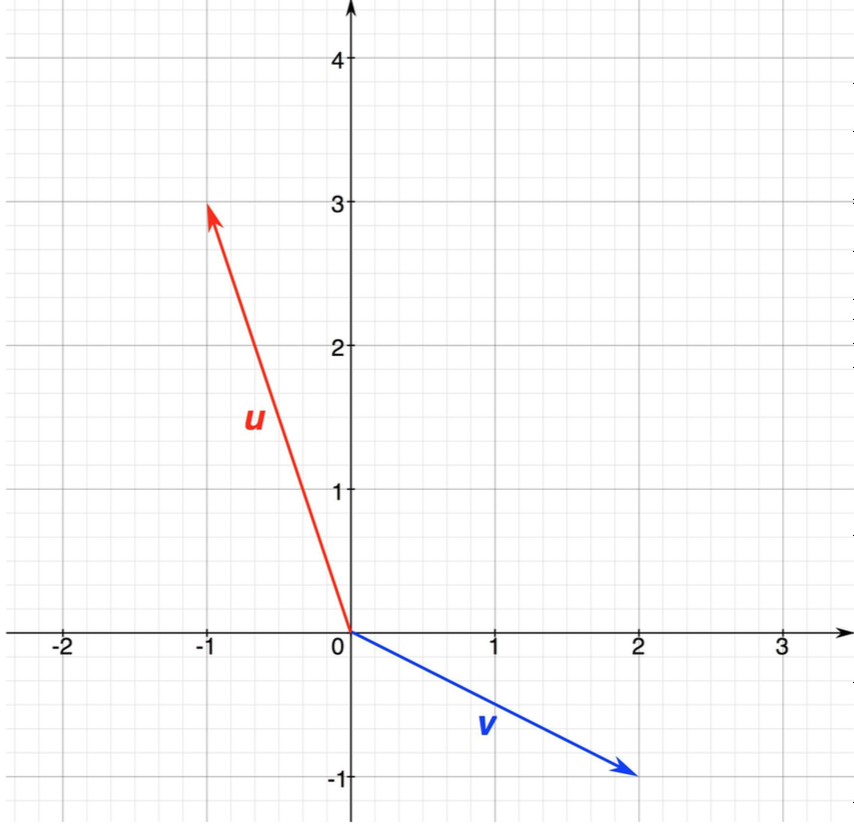
It just so happens that in our case these vectors are faces.
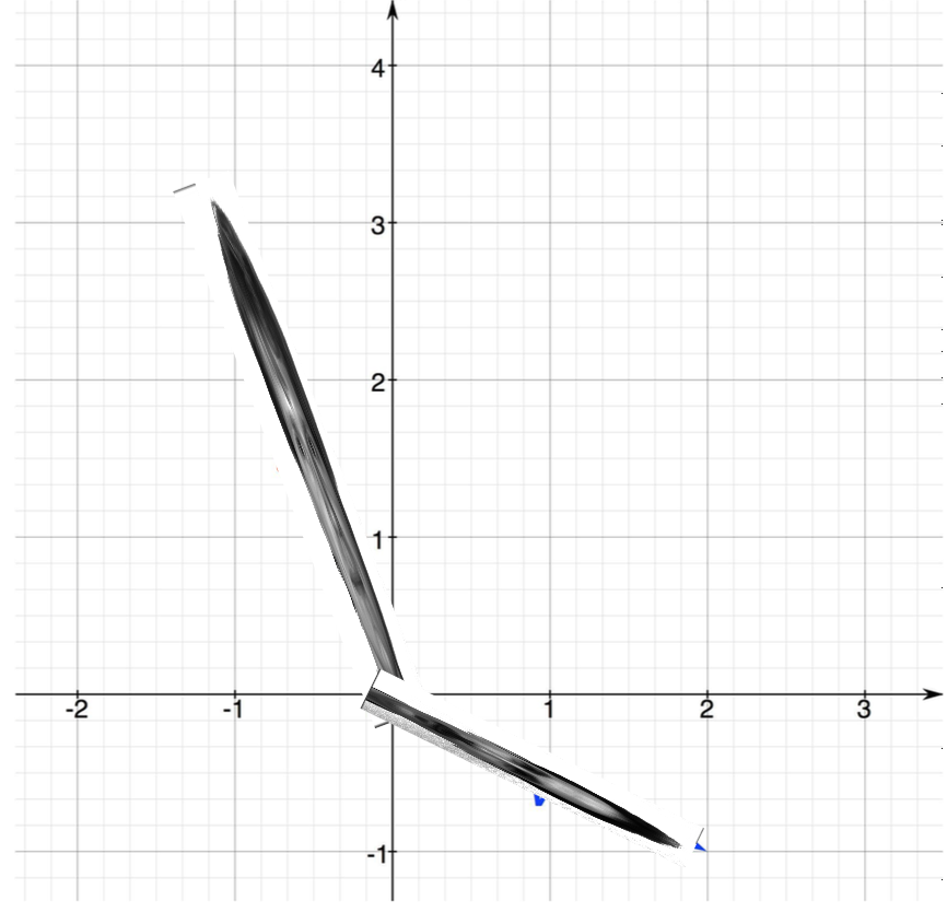
These faces are independent and they span the plane because we have two of them, but the basis that they form is not intuitive or easy to use. What I mean by this is that if I want to get to point (1,1) in this space I need \(- \frac{4}{5}v + (-\frac{13}{5})u\). Whereas, if \(v\) was the the unit vector along the x axis and \(u\) was the unit vector along the y axis we would only need \((1)v + (1)u\) in order to get to position (1,1). Well the columns of \(U\), or eigenfaces as they are colloquially known, represent this “nice” basis.
With this subspace in mind we can now represent any face vector in our 77760 dimensional space as a linear combination of the eigenface basis. To find the weights of this linear combination, the amount that each eigenface contributes to any given face, each face is projected onto the eigenface space
\[(\Gamma - \Psi)^TU = [w_1,w_2,...,w_d] = W\]The amount that each eigenface contributes to this linear combination is the feature representation that we will use for our images. Now to perform classification we will use a 1-nearest neighbors classifier. This is done by finding the face in our training set that is closest to our unknown face.
\[\arg \min_i \|W-W_i\|\]# Split into training and test set
x_train, x_test, y_train, y_test = train_test_split(faces.T, labels, test_size=0.3)
# Put the faces in the columns of x_train
x_train = x_train.T
x_test = x_test.T
# Train with knn=1 and dimensionality of 34
d = 34
k = 1
# Subtract off the mean
mean_face = np.mean(x_train, axis=1)
x_train = x_train - mean_face
# Find low dimensional subspace using PCA
pca = PCA(n_components=d)
pca.fit(x_train)
model = pca.transform(x_train)
# Project the known faces onto the face space
label_map = np.dot(x_train.T, model)
# Train a KNN classifier
knn = KNeighborsClassifier(n_neighbors=k)
knn.fit(label_map, y_train)
# project the unknown faces onto face space
W = np.dot(x_test.T - mean_face.T, model)
# Predict the unknown faces
print "precision test: ", metrics.precision_score(y_test, knn.predict(W))
This yields a classifier that is 80% precise! So we’re done right?
What’s Next? (Learning Curves)
Well, that depends on if 80% is good enough. If it is yes, we’re done but if we need more precision, or more of whatever metric you are optimizing for we need to do something else. That something else is trying to diagnose where our learning algorithm is falling short. When it comes to learning there are a few things that we can change, the data, the features, or the model. Almost universally more data improves the performance of the learning algorithm but most of the time collecting more data isn’t possible. The next thing that we can change is the features we could try more, fewer, or different features Lastly we could change the model, make it more flexible, less flexible, play with the regularizer, but the problem still remains how to choose which course of action to take? I like to use learning curves.
A learning curve is a plot of the training performance vs the cross validation (testing) performance as the size of the training set increases. They can help guide us toward what we need to change in order to improve our learning system. Learning curves help us identify whether our algorithm suffers from high bias or high variance. High bias occurs when both the training and test performance are low. In the diagram below the training performance is the blue line and the testing performance is the green line.
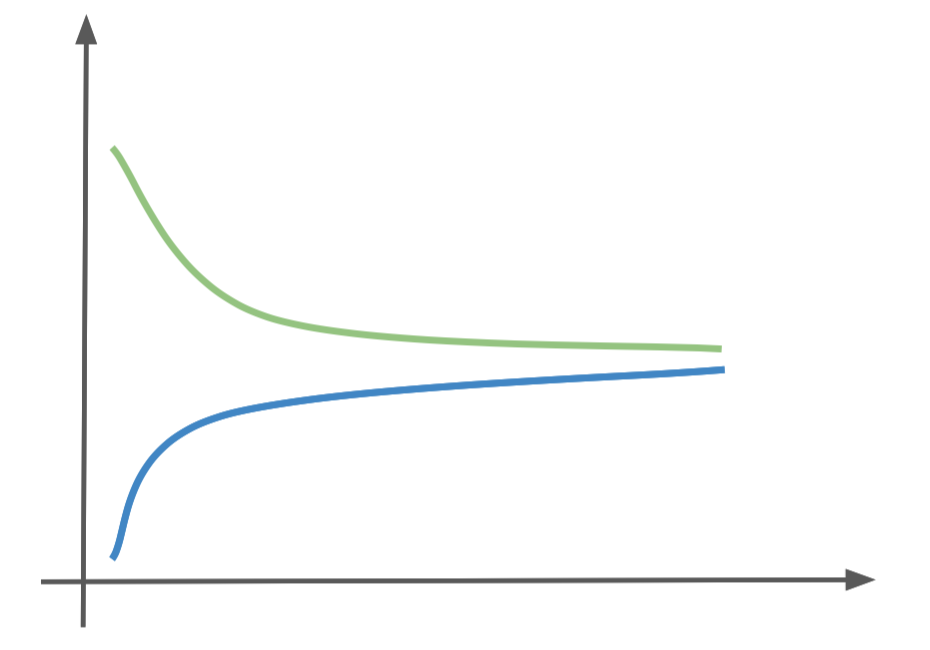
The other common problem is high variance, or over-fitting, where the model matches the training set too well and does not generalize to unseen examples. This is evident when there is a large gap between the training and testing performance.
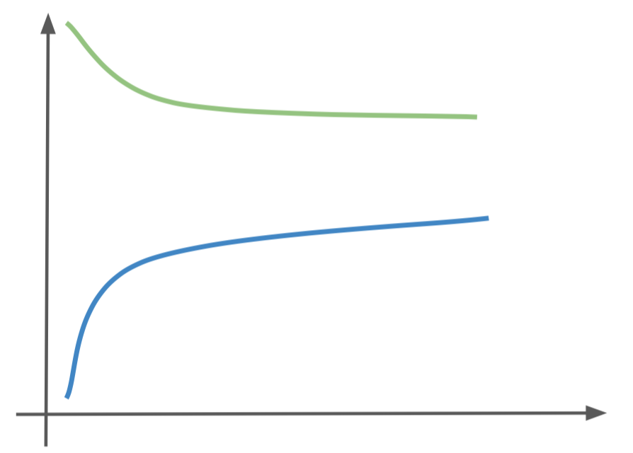
We can generally help the high bias problem by using more features, different features, playing with regularization, or changing the model. We can help over fitting by using fewer features, getting more data, changing the model to a less expressive one, or changing the regularization. Let’s take a look at the learning curves for our classifier and see what we can do to improve our system.
def learning_curve_mod(data, labels, clf, percents, d=100, avg=3, test_size=.2):
    """
    This method calculates the performance of the training and cross validation test set as the training
    set size increases and returns the performance at each percent

    Args:
        :param data: (md.array) The raw data to use for training and cross validation testing
        :param labels: (nd.array) the labels associated with the data
        :param clf: (sklearn classifier) the classifier to be used for training
        :param percents: (nd.array) a list of percent of training data to use
        :param d:  (int) The number of principle components to calculate
        :param avg: (int) The number of iterations to average when calculating performance
        :param test_size: (double [0,1]) The size of the testing set

    Return:
        :return: train_accuracies (list) performance on the training set
        :return: test_accuracies (list) performance on the testing set
    """
    # split into train and testing dataset
    x_train, x_test, y_train, y_test = train_test_split(data.T, labels, test_size=test_size, random_state=0)
    x_test = x_test.T
    train_accuracies = []
    test_accuracies = []
    for percent in percents:
        temp_train_accuracies = []
        temp_test_accuracies = []
        print percent
        for i in range(0, avg):
            x_train_2, x_test_2, y_train_2, y_test_2 = train_test_split(x_train, y_train, test_size=percent)
            x_train_2 = x_train_2.T

            # Subtract off the mean
            mean_face = np.mean(x_train_2, axis=1)
            x_train_2 = x_train_2 - mean_face

            # Find low dimensional subspace using PCA
            pca = PCA(n_components=d)
            pca.fit(x_train_2)
            model = pca.transform(x_train_2)

            # Project the known faces onto the face space
            label_map = np.dot(x_train_2.T, model)

            # Train a KNN classifier
            clf.fit(label_map, y_train_2)

            # project the unknown faces onto face space
            W_train = np.dot(x_train_2.T - mean_face.T, model)
            W_test = np.dot(x_test.T - mean_face.T, model)


            test_prediction = clf.predict(W_test)
            temp_test_accuracies.append(metrics.precision_score(y_test, test_prediction))
            train_prediction = clf.predict(W_train)
            temp_train_accuracies.append(metrics.precision_score(y_train_2, train_prediction))

        train_accuracies.append(np.mean(temp_train_accuracies))
        test_accuracies.append(np.mean(temp_test_accuracies))

    return train_accuracies, test_accuracies

# =============================================================================
# Learning curve on initial machine learning k=1, d=32
# =============================================================================
percents = np.linspace(0, .6, 15)[::-1]  # backwards
d = 32
k = 1
clf = KNeighborsClassifier(n_neighbors=k)
train_accuracies, test_accuracies = learning_curve_mod(x_train, y_train, clf, percents, d=d)
test_plot = plt.plot(1 - percents, test_accuracies, label="Test")
train_plot = plt.plot(1 - percents, train_accuracies, 'g-', label="Train")
plt.xlabel("Percent of training data used")
plt.ylabel("Model Precision")
plt.title("Learning Curve (KNN) d=" + str(d) + ", k=" + str(k))
plt.ylim([0, 1.1])
plt.legend(loc=4, markerscale=2, fontsize=20)
plt.show()
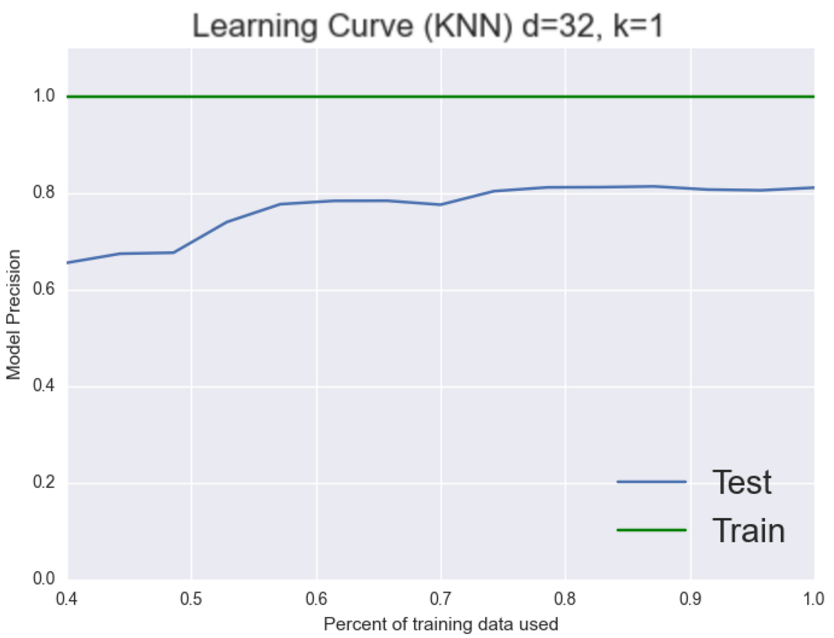
As you can see it appears that we have a high variance problem. The training set is always around 100% whereas the testing set is stuck at 80%. So we have a system that is performing very well on the training set but not as well as we’d like on the testing set which implies that we could be over-fitting. Let’s choose a more stringent model like 2-nearest neighbors and see if that fixes our over-fitting problem.
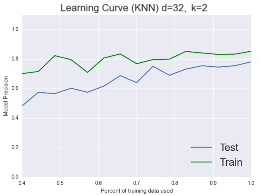
It appears to! As we’d expect now our model seems to generalize better. Both the training and testing set are increasing together to about the same place. It’s still not high enough but now we can see that our problem is a bias one. Let’s see if we can add more features to fix this problem.
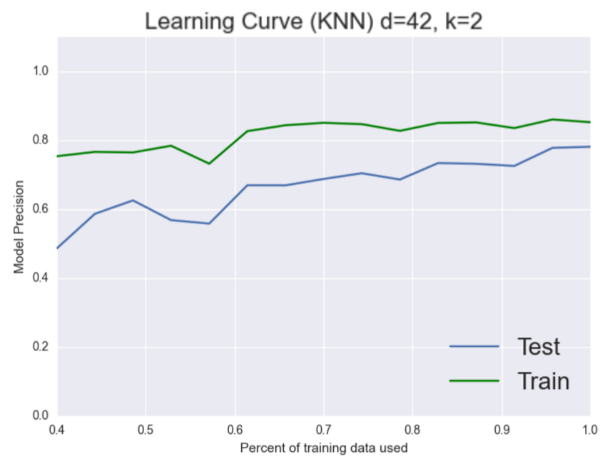
Nope, it doesn’t look like more features helped here, which is fine we’re trying to debug this thing. Nothing that we try is gauranteed to work. Let’s try and choose a better model. KNN is a pretty naive model perhapse logistic regression can give us better results
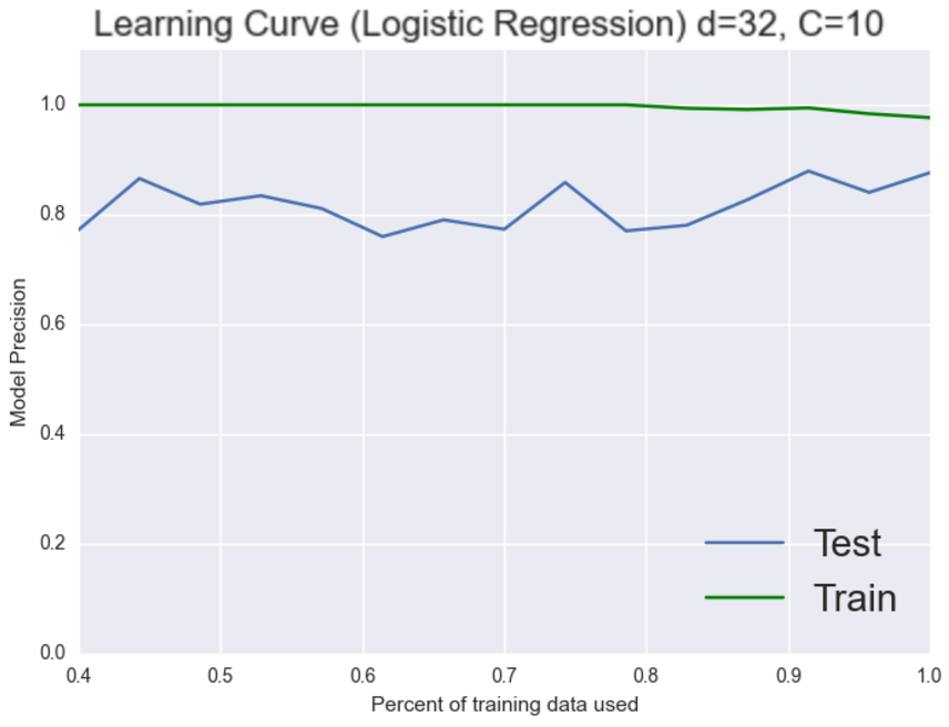
Wow, we just jumped 7% that’s pretty good. We’re back to scoring perfectly on the training set though. However this time both classifiers are doing really well so now it gets a bit trickier. It could be either the bias or the variance that is still causing this system problems. Working on the bias seemed to give us good results last time let’s try to add more features again and see what happens.
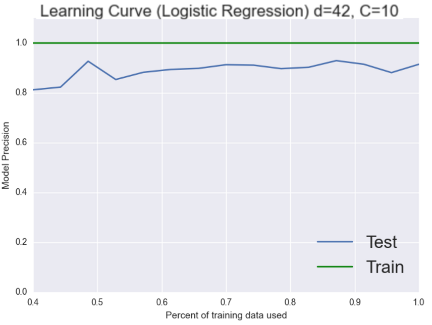
Excellent, our systme is now performing in the 90’s! We just imporved our system by over 10% in a few minutes by examining learning curves and thinking critically about how to adjust our system. Hopefully you learned a bit about additional system tuning from this short essay. All of the code for today is available here