Introduction to Bayesian Networks
Introduction
The goal of graphical models is to represent some joint distribution over a set of random variables. In general this is a difficult problem, because even if our random variables are binary, either 1 or 0, our model will require an exponential number of assignments to our values (\(2^n\)). By using a graphical model we can try to represent independence assumptions and thus reduce the complexity of our model while still retaining its predictive power. In this tutorial I’m going to talk about Bayesian networks, which are a type of directed graphical model where nodes represent random variables and the paths represent our independence assumptions. I’ll go over the basic intuition and operations needed, and build a simple medical diagnosis model. The point of this tutorial is not to discuss all of the ways to reason about influence in a Bayes net but to provide a practical guide to building an actual functioning model. Let’s get started.
Motivating example
Imagine that we are doctors and we want to predict whether or not a patient will have a heart attack. We have a few pieces of information that we can collect like the patients cholesterol, whether or not they smoke, their blood pressure, and whether or not they exercise. Now in order to describe this system fully we would need \(2^5\) interactions. However, this many interactions might not lend itself to any additional predictive power. We’re doctors and we know some things about this disease. For example, we know that blood pressure is directly related to heart attacks and that both exercise and smoking can affect blood pressure. Thus we can build a model like the one in Figure 1 where we use our domain knowledge to describe the interactions between our features.
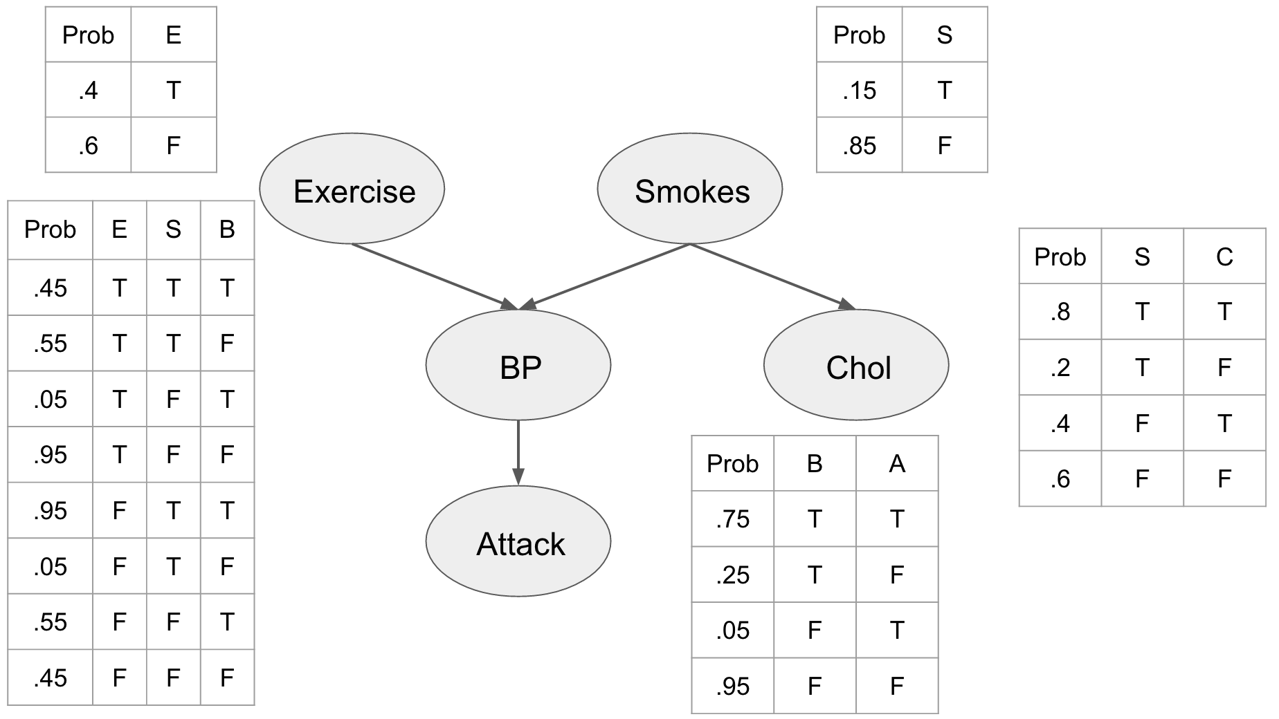
This picture shows us a number of things about our problem and our assumptions. First off we see the prior probabilities of the individual being a smoker, and whether or not they exercise. We can see that being a smoker affects the individuals cholesterol level influencing whether it is either high (T) or low (F). We also see that the blood pressure is directly influenced by exercise and smoking habits, and that blood pressure influences whether or not our patient is going to have a heart attack.
We assume that this network represents the joint distribution \(P(E, S, C, B, A)\) and by describing these relationships explicitly we can use the chain rule of probability to factorize it as:
\begin{align} P(E, S, C, B, A) &= P(E)P(S)P(C | S)P(B|E,S)P(A|B) \end{align}
Now let’s explore how we might use this network to make predictions about our patient. Let’s figure out the probability of a patient exercising regularly, not smoking, not having high cholesterol, not having high blood pressure, and not getting a heart attack. This is easy we just look at our conditional probability tables (CPTs).
\begin{align} P(E=T, S=F, C=F, B=F, A=F) &= P(E=T)P(S=F)P(C=F | S=F)P(B=F|E=T,S=F)P(A=F|B=F)\newline &= .4\times .85 \times .6 \times .95 \times .95\newline &= .184 \end{align}
This is useful but the real power of the Bayesian network comes from being able to reason about the whole model, and the effects that different variable observations have on each other. In order to perform this inference we’ll need three operations, variable observation, marginalization, and factor products.
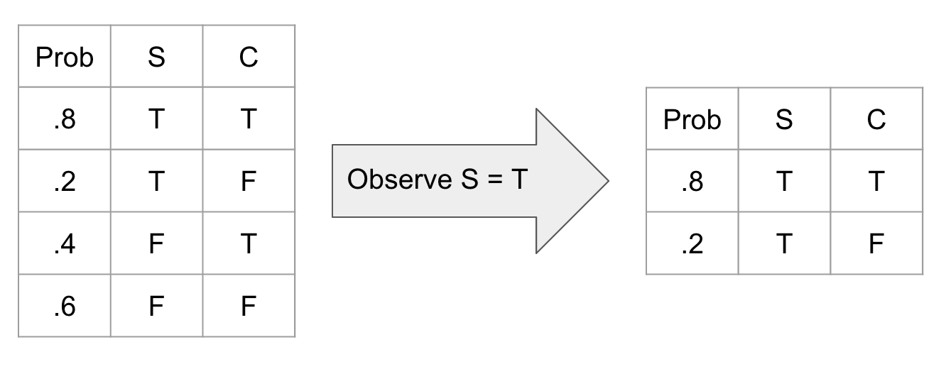
Observing a variable is a simple operation where we just ignore all unobserved aspects of that variable. This translates into deleting all rows of a CPT where that observation is not true.
or in python
def observe(network, var_name, observation):
"""
Observes a given variable in our network. This just deletes all entries not consistent
with the observation
Args:
:param network: (list pandas.dataframe) list of the cpts in the network
:param var_name: (list string) name of the observed variables
:param observation: (list string) values that are observed
Returns:
:return: (pandas.dataframe)
"""
observed_network = []
for cpt in network:
for var,obs in zip(var_name, observation):
if var in cpt.columns:
cpt = cpt[cpt[var] == obs]
observed_network.append(cpt)
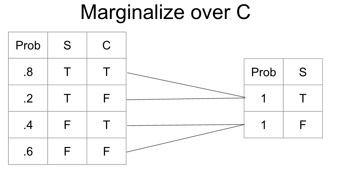
return observed_networkMarginalization is the process of changing the scope of a CPT by summing over the possible configurations of the variable to eliminate. It gives us a new probability distribution irrespective of the variable that we marginalized.
def marginalize_factor(cpt, factor):
"""
This method marginalizes out a single factor by summing over all possible value combinations for that factor
"""
# Drop the factor to be marginalized out
probs = cpt["probs"]
cpt = cpt.drop([factor, "probs"], axis=1)
# Create a new table to store marginalized values
marginalized_cpt = pd.DataFrame(columns=list(cpt.columns))
marginalized_probs = []
# Marginalize the cpt
while cpt.shape[0] > 0:
# Find all positions that have the same feature pattern
positions = [x for x in range(0, cpt.shape[0]) if sum(cpt.iloc[0] == cpt.iloc[x]) == cpt.shape[1]]
# Sum up all probabilities
marginalized_probs.append(sum(probs[probs.index[positions]]))
# add the factor configuration to the marginalized cpt
marginalized_cpt = marginalized_cpt.append(cpt[:1])
# Drop all positions that have been summed
cpt = cpt.drop(cpt.index[positions], axis=0)
probs = probs.drop(probs.index[positions], axis=0)
#marginalized_cpt["probs"] = marginalized_probs
marginalized_cpt.insert(0, "probs", marginalized_probs)
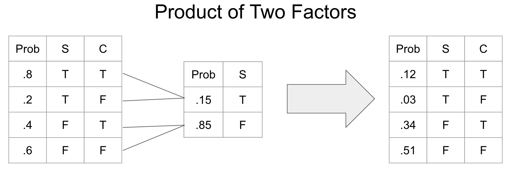
return marginalized_cptA factor product is a way of joining two CPTs into a new CPT.
def factor_product(cpt1, cpt2):
    """
    This method takes the factor product of two cpts by multiplying where the variables overlap

    Args:
        :param cpt1: (pandas.DataFrame)
        :param cpt2: (pandas.DataFrame)

    Returns:
        :returns cpt: (pandas.DataFrame)
    """
    # Find the names of all columns
    column_names = list(set(cpt1.columns).union(set(cpt2.columns)).difference(set(["probs"])))
    shared_features = list(set(cpt1.columns).intersection(set(cpt2.columns)).difference(set(["probs"])))
    probs = []

    # Create an empty data frame to store the product cpt table
    cpt = pd.DataFrame(columns=column_names)
    idx = 0
    for i in range(0, cpt1.shape[0]):
        for j in range(0, cpt2.shape[0]):
            if sum(cpt1[shared_features].iloc[i] == cpt2[shared_features].iloc[j]) == len(shared_features):
                probs.append(cpt1["probs"].iloc[i] * cpt2["probs"].iloc[j])
                vals = []
                for name in column_names:
                    if name in cpt1.columns:
                        vals.append(cpt1[name].iloc[i])
                    else:
                        vals.append(cpt2[name].iloc[j])
                cpt.loc[idx] = vals
                idx = idx + 1

    cpt.insert(0, "probs", probs)
    return cpt
In this tutorial we are going to perform exact inference because our networks are fairly small. We will use the method of Variable elimination to make predictions in our network. The outline of the procedure is as follows
-
Observe variables
-
For each variable that we want to marginalize out
a. Product all CPT’s containing said variable
b. marginalize the variable out fo the combined CPT
-
Join all remaining factors
-
Normalize
def infer(network, marg_vars, obs_vars, obs_vals):
    """
    This function performs inference on a bayesian network

    Args:
        :param network: (list pandas.DataFrame)
        :param marg_vars: (list string)
        :param obs_vars: (list string)
        :param obs_vals: (list int)

    Returns:
        :returns:
    """
    # Observe variables
    network = observe(network, obs_vars, obs_vals)

    # while there are still variables to be marginalized
    for marg_var in marg_vars:
        marg_net = []
        rm_nodes = []
        for i, node in enumerate(network):
            if marg_var in node.columns:
                marg_net.append(node)
                rm_nodes.append(i)

        # Check to see if marg_vars is present
        if not len(marg_net) == 0:
            table = marg_net[0]

            # delete marginalized nodes from network
            rm_nodes.reverse()
            for rm in rm_nodes:
                del network[rm]

            # marginalize out variables
            for cpt in marg_net[1:]:
                table = factor_product(table, cpt)

            marginalized_table = marginalize_factor(table, marg_var)
            network.append(marginalized_table)

    # When all variables have been marginalized product the table together
    product = network[0]
    for node in network[1:]:
        product = factor_product(product, node)

    # Normalize
    product["probs"] = product["probs"] / sum(product["probs"])

    return product
Let’s use these methods to analyze how information flows in our network. We can instantiate our bayesian network as:
chol = create_cpt(["s", "c"], [.8, .2, .4, .6], [(1, 0), (1, 0)])
smoke = create_cpt(["s"], [.15, .85], [(1, 0)])
bp = create_cpt(["e", "s", "b"],
                [.45, .55, .05, .95, .95, .05, .55, .45],
                [(1, 0), (1, 0), (1, 0)])
exercise = create_cpt(["e"], [.4, .6], [(1, 0)])
attack = create_cpt(["b", "a"], [.75, .25, .05, .95], [(1, 0), (1, 0)])
heart_net = [exercise, smoke, chol, bp, attack]
Let’s assume that all we know about the patient is that he is a smoker. What does that do to the probability that he will have a heart attack?
infer(heart_net, ["c", "b", "e", "s"], ["s"], [1])| probs | a | |
|---|---|---|
| 0 | 0.575 | 1 |
| 1 | 0.425 | 0 |
As we would expect it increases. This is what is known as causal reasoning, because influence flows from the contributing cause (smoking) to one of the effects (heart attack). There are other ways for information to flow though. For example, let’s say that we know that the patient had a heart attack. Unfortunately, since they are now dead we can’t measure their blood pressure directly, but we can use our model to predict what the probability of them having high blood pressure is.
infer(heart_net, ["c", "a", "e", "s"], ["a"], [1])| probs | b | |
|---|---|---|
| 0 | 0.912463 | 1 |
| 1 | 0.087537 | 0 |
Clearly having a heart attack suggests that the patient was likely to have had high blood pressure. This is an example of what is known as evidential reasoning. We used the evidence of a heart attack to better understand the patients initial state.
The last form of reasoning in these types of networks is known as intercausal reasoning. This is where information flows between two otherwise independent pieces of evidence. Take for example whether or not the patient exercises or smokes. If we observe that the patient has high blood pressure then the probability that he either smokes or doesn’t exercise increases.
infer(heart_net, ["c", "a", "b"], ["b"], [1])| probs | s | e | |
|---|---|---|---|
| 0 | 0.065854 | 1 | 1 |
| 1 | 0.041463 | 0 | 1 |
| 2 | 0.208537 | 1 | 0 |
| 3 | 0.684146 | 0 | 0 |
If we then observe that the patient doesn’t exercise we see that the probability that he is a smoker jumps substantially.
infer(heart_net, ["c", "a", "b", "e"], ["b", "e"], [1, 1])| probs | s | |
|---|---|---|
| 0 | 0.613636 | 1 |
| 1 | 0.386364 | 0 |
This is an example of information flowing between two previously independent factors! I have created an IPython notebook so that you can play with these ideas if you’d like located here.