Label Smarter Not More

Introduction
Imagine back to your school days studying for an exam. Did you randomly read sections of your notes, or randomly do problems in the back of the book? No! Well, at least I hope you didn’t approach your schooling with the same level of rigor as what to eat for breakfast. What you probably did was figure out what topics were difficult for you to master and worked diligently at those. Only doing minor refreshing of ideas that you felt you understood. So why do we treat our machine students differently?
We need more data! It is a clarion call I often hear working as a Data Scientist, and it’s true most of the time. The way this normally happens is some problem doesn’t have enough data to get good results. A manager asks how much data you need. You say more. They hire some interns or go crowdsource some labelers, spend a few thousand dollars and you squeak out a bit more performance. Adding in a single step where you let your model tell you what it wants to learn more about can vastly increase your performance with a fraction of the data and cost. I’m talking about doing some, get ready for the buzz word, active learning.
In this article, we will run some basic experiments related to active learning and data selection. We will train a random forest on a small subset of the IMDB Sentiment dataset. Then we will increase the training set by sampling randomly, and by sampling data points that the model wants to learn about. We will compare our performance increase with respect to increasing data and show how smart labeling can save time, money, and increase performance. The code for this project is in a gist here, and also included at the bottom of this article. Let’s get started.
Appeal to Reader
If you pay for Medium, or haven’t used your free articles for this month, please consider reading this article there. I post all of my articles here for free so everyone can access them, but I also like beer and Medium is a good way to collect some beer money : ). So please consider buying me a beer by reading this article on Medium.
TLDR
If your problem needs more data, try labeling it with the help of your classifier. Do this by either choosing the examples with the least confidence or the examples where the highest and second-highest probabilities are closest. This works most of the time but is no panacea. I’ve seen random sampling do as well as these active learning approaches.
The Data
For this problem, we will be looking at the IMDB Sentiment dataset and trying to predict the sentiment of a movie review. We are going to take the whole test set for this dataset, and a tiny subset of training data. We’ll gradually increase the training set size based on different sampling strategies and look at our performance increase.
There are about 34,881 examples in the training set and only 15,119 in the test set. We start by loading the data into a pandas data frames.
df = pd.read_csv("IMDB_Dataset.csv")
df["split"] = np.random.choice(["train", "test"], df.shape[0], [.7, .3])
x_train = df[df["split"] == "train"]
y_train = x_train["sentiment"]
x_test = df[df["split"] == "test"]
y_test = x_test["sentiment"]
Basic Model
For this tutorial, we’ll look at a simple Random Forest. You can apply these techniques to just about any model you can imagine. The model only needs a way of telling you how confident it is in any given prediction. Since we’re working with text data our basic model will use TF-IDF features from the raw text. I know, I know, we should use a deep transformer model here, but this is a tutorial on active learning not on SOTA so forgive me. If you want to see how to use something like BERT check out my other tutorial here.
We’ll define our RandomForest model as a SciKit-Learn pipeline using only unigram features:
from sklearn.ensemble import RandomForestClassifier
from sklearn.pipeline import Pipeline
from sklearn.feature_extraction.text import TfidfVectorizer
clf = RandomForestClassifier(n_estimators=100, random_state=0)
model = Pipeline(
            [
                ("tfidf", TfidfVectorizer(ngram_range=(1,1))),
                ("classifier", clf),
            ]
        )
Now we can call .fit() on a list of text input and the pipeline will handle the rest. Let’s use our initial training set of 5 examples and see how we do on the test set.
# Get five random examples for training.
rand_train_df = x_train.sample(5)
model.fit(rand_train_df["review"], rand_train_df["sentiment"])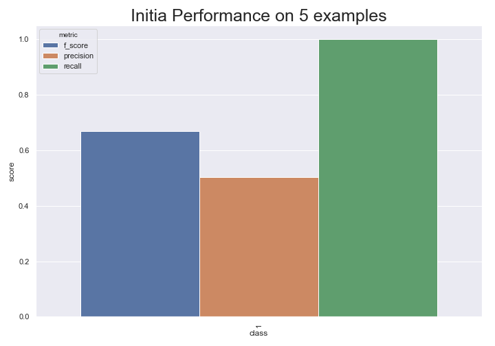
From this, we can see the dataset is pretty balanced since predicting all positive gives us almost .5 precision. This model is pretty crappy though since it only predicts positive. Let’s see if we can use active learning to get to better performance faster than randomly sampling new points.
Choosing Good Data Points to Label
So we have a classifier now. It’s meh at best, and we want more data. Let’s use the classifier to make predictions on our other training data and see which points the model is least confident about. For most Sci-Kit Learn estimators this is super easy. We can use the .predict_proba() function to get a probability for each class. To do this by hand you could also look at the individual predictions of the trees and count the votes for each class. However, predict_proba is much more convenient : ).
preds = model.predict_proba(x_test["review"])This will give us a numpy array of probabilities where each column is a class and each row is an example. It’s something like:
[[.1, .9],
 [.5, .5],
 [.2, .8]...
Uncertainty Sampling
The simplest “intelligent” strategy for picking good points to label is to use the points which the model is least confident about. In the example above that would be the second point, because the maximum probability of any class is the smallest.
def uncertainty_sampling(df, preds, n):
    """samples points for which we are least confident"""
    df["preds"] = np.max(preds, axis=1)
    return df.sort_values("preds").head(n).drop("preds", axis=1)
Here we have a function that takes a data frame of training examples, the associated predicted probabilities, and the number of points we want to sample. It then gets the maximum value in each row, sorts the data points from smallest to largest, and grabs the n examples that had the smallest maximum probability.
If we apply uncertainty sampling to the three example probabilities above we’d say we should label [.5, .5] first because the maximum probability is smaller than all the other maximum probabilities. (.8 and .9) which intuitively makes sense!
Margin Sampling
Uncertainty sampling is nice, but in the multiclass setting, it doesn’t do as good of a job of capturing uncertainty. What if you had the following predictions?
[[.01, .45, .46],
 [.28, .28, .44],
 [0.2, 0.0, .80]...
The data point which the model seems to be most uncertain about is the first one since it’s predicting class 3 by just .01! But Uncertainty sampling would say that example two is the best point to label since .44 is the smallest maximum probability. They are both good candidates, but the first intuitively makes more sense. Margin sampling caters to this intuition; that the best points to label are those with the smallest margin between predictions. We can perform margin sampling with the following function:
def margin_sampling(df, preds, n):
    """Samples points with greatest difference between most and second most probably classes"""
    # Sort the predictions in increasing order
    sorted_preds = np.sort(preds, axis=1)

    # Subtract the second highest prediction from the highest
    # We need to check if the classifier has more than one class
    if sorted_preds.shape[1] == 1:
        return df.sample(n)
    else:
        df["margin"] = sorted_preds[:, -1] - sorted_preds[:, -2]
        return df.sort_values("margin").head(n).drop("margin", axis=1)
In this code, we sort the predicted probabilities. Then we check to see if the array has more than one dimension. If it has only one probability it only saw one class and has no information about the existence of other classes. In this case, we need to just randomly sample. Otherwise, we find the margin by subtracting the second-highest probability from the highest probability and sorting the results.
Experiments
I ran a simple experiment where I start with five randomly sampled points, then apply each sampling strategy to gain five more points. I do this iteratively 100 times until I’ve sampled about 500 points. I plot the f1 score on the test set at each time point and look at how our performance improves with each sampling strategy.
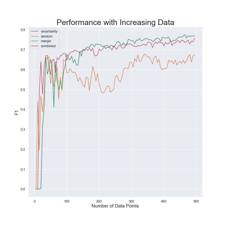
You can see that Marginal Sampling and Uncertainty sampling both do better than random for this problem. They are the same in the binary classification case I didn’t think about this when I started writing this article 😅. I created an additional sampling strategy called combined which does a little bit of margin sampling, a little bit of uncertainty sampling, and a little bit of random sampling. I like this combined approach for many of my projects because sometimes random sampling does help. If we are always sampling according to the margin, or uncertainty, we aren’t sampling uniformly from our dataset and could be missing out on some important information. Anecdotally, I’ve seen a little random in the sampling usually pays off. Though don’t believe me because I haven’t run any good experiments to prove this yet 😅.
Conclusion
Active learning can help you get better performance with fewer data by choosing new points that add the most information to your model. This strategy works pretty well most of the time but isn’t guaranteed to do better. It’s a nice tool to keep in mind when you’re thinking about labeling some additional data.
Code
from typing import Dict, List

import matplotlib.pyplot as plt
import numpy as np
import pandas as pd
import seaborn as sns
from sklearn.ensemble import RandomForestClassifier
from sklearn.feature_extraction.text import TfidfVectorizer
from sklearn.pipeline import Pipeline
sns.set()

def uncertainty_sampling(df: pd.DataFrame, preds: np.array, n: int) -> pd.DataFrame:
    """samples points for which we are least confident"""
    df["preds"] = np.max(preds, axis=1)
    return df.sort_values("preds").head(n).drop("preds", axis=1)

def random_sampling(df: pd.DataFrame,  preds: np.array, n: int) -> pd.DataFrame:
    return df.sample(n)

def margin_sampling(df: pd.DataFrame,  preds: np.array, n: int) -> pd.DataFrame:
    """Samples points with greatest difference between most and second most probably classes"""
    # Sort the predictions in increasing order
    sorted_preds = np.sort(preds, axis=1)

    # Subtract the second highest prediction from the highest prediction
    # We need to check if the classifier has more than one class here.
    if sorted_preds.shape[1] == 1:
        return df.sample(n)
    else:
        df["margin"] = sorted_preds[:, -1] - sorted_preds[:, -2]
        return df.sort_values("margin").head(n).drop("margin", axis=1)

def combined_sampling(df: pd.DataFrame,  preds: np.array, n: int, weights: List[float]=None) -> pd.DataFrame:
    """weighted sample with random, margin, and uncertainty"""
    if weights is None:
        weights = [.4, .4, .2]

    margin_points = margin_sampling(df, preds, round(n * weights[0]))
    uncertainty_points = uncertainty_sampling(df, preds, round(n * weights[1]))

    # Resample the dataframe and preds to remove the sampled points
    remaining_df = df.iloc[~(df.index.isin(margin_points.index) | df.index.isin(uncertainty_points.index))]
    random_points = random_sampling(remaining_df, preds, round(n * weights[0]))
    final_df = pd.concat([random_points, uncertainty_points, margin_points]).drop_duplicates().head(n)
    print(final_df.shape)
    return final_df

def evaluate_model_improvement(model,
                               train_df: pd.DataFrame,
                               test_df: pd.DataFrame,
                               sample_func,
                               n: int,
                               label_col: str,
                               data_col: str,
                               random_state: int=1234,
                               num_iterations: int=30
                              ) -> List[Dict[str, Dict[str, float]]]:
    train_data = train_df.sample(n, random_state=random_state)
    scores = []
    for i in range(1, num_iterations, 1):
        # Clone the model to make sure we don't reuse model state
        model = sklearn.base.clone(model)

        # fit the model on our data
        model.fit(train_data[data_col], train_data[label_col])

        # Get predictions for the current data level
        preds = model.predict(test_df[data_col])
        scores.append(classification_report(test_df[label_col], preds, output_dict=True))

        # Get all points in training set that haven't been used
        remaining_df = train_df.iloc[~train_df.index.isin(train_data.index)]

        # Resample the data
        new_samples = sample_func(remaining_df, model.predict_proba(remaining_df[data_col]), n)
        train_data = pd.concat([train_data, new_samples])

    return scores

# Load in the data
df = pd.read_csv("IMDB_Dataset.csv")
df["split"] = np.random.choice(["train", "test"], df.shape[0], [.7, .3])
x_train = df[df["split"] == "train"]
y_train = x_train["sentiment"]
x_test = df[df["split"] == "test"]
y_test = x_test["sentiment"]

# Sample each point
uncertainty_scores = evaluate_model_improvement(model, x_train, x_val, uncertainty_sampling, 5,
                                                "sentiment", "review", rand_state, num_iterations=100)
random_scores = evaluate_model_improvement(model, x_train, x_val, random_sampling, 5,
                                           "sentiment", "review", rand_state, num_iterations=100)
margin_scores = evaluate_model_improvement(model, x_train, x_val, margin_sampling, 5,
                                           "sentiment", "review", rand_state, num_iterations=100)
combined_scores = evaluate_model_improvement(model, x_train, x_val, combined_sampling, 5,
                                             "sentiment", "review", rand_state, num_iterations=100)

fig, ax = plt.subplots(1, 1, figsize=(10, 10))
key = "positive"
x_points = np.cumsum([5] * 99)
plt.plot(x_points, np.array([x[key]["f1-score"] for x in uncertainty_scores]), label="uncertainty")
plt.plot(x_points, np.array([x[key]["f1-score"] for x in random_scores]), label="random")
plt.plot(x_points, np.array([x[key]["f1-score"] for x in margin_scores]), label="margin")
plt.plot(x_points, np.array([x[key]["f1-score"] for x in combined_scores]), label="combined")
handles, labels = ax.get_legend_handles_labels()
ax.legend(handles, labels)
ax.set_title("Performance with Increasing Data", fontsize=25)
ax.set_xlabel("Number of Data Points", fontsize=15)
ax.set_ylabel("F1", fontsize=15)