Good Grams: How to Find Predictive N-Grams for your Problem

Introduction
Nowadays NLP feels like it’s just about applying BERT and getting state of the art results on your problem. Often times, I find that grabbing a few good informative words can help too. Usually, I’ll have an expert come to me and say these five words are really predictive for this class. Then I’ll use those words as features, and voila! You get some performance improvements or a little bit more interpretability. But what do you do if you don’t have a domain expert? One easy thing I like to try is to train a simple linear model on the TF-IDF features and take the top n words or n-grams : ).
In this blog post we’ll:
-
Train a simple model using SciKit-Learn and get the most informative n-gram features
-
Then run some performance comparisons on models with different numbers of features.
By the end of this tutorial hopefully, you’ll have a fun new tool for uncovering good features for text classification. Let’s get started.
Appeal to Reader
If you pay for Medium, or haven’t used your free articles for this month, please consider reading this article there. I post all of my articles here for free so everyone can access them, but I also like beer and Medium is a good way to collect some beer money : ). So please consider buying me a beer by reading this article on Medium.
TLDR
Use a linear classifier on SciKit-Learn’s TfidfVectorizer then sort the features by their weight and take the top n. You can also use the TfidfVectorizer to extract only a subset of n-grams for your model by using the vocabulary parameter.
Motivation
One very successful way to classify text is to look for predictive words, or short phrases, that are relevant to the problem. In the context of say movie review sentiment, we could look for the words “good”, “excellent”, “great”, or “perfect” to find good reviews and “bad”, “boring”, or “awful” to find bad reviews. As subject matter experts in good and bad movie reviews, it was easy for us to come up with these features.
More often than not, I am not a subject matter expert and it’s hard for me to determine what good predictive words or phrases might be. When this happens, and I have labeled data, there is a quick way to find descriptive words and phrases. Just train a linear model and sort the weights!
Build the Bot
We have data , a model that has been trained on our data, and a Twitter developer account all that is left is to link them together. Our bot needs to do 3 things.
-
Authenticate with the Twitter API
-
Generate a proverb
-
Post that proverb to Twitter.
Luckily Tweepy makes the first and third part super easy and we’ve already done the second!
Train a Simple Model
SciKit-Learn makes it very easy to train a linear model and extract the associated weights. Let’s look at training a model on the IMDB sentiment dataset.
df = pd.read_csv("IMDB_Dataset.csv")
df["split"] = np.random.choice(["train", "val", "test"], df.shape[0], [.7, .15, .15])
x_train = df[df["split"] == "train"]
y_train = x_train["sentiment"]
x_val = df[df["split"] == "val"]
y_val = x_val["sentiment"]
classifier = svm.LinearSVC(C=1.0, class_weight="balanced")
tf_idf = Pipeline([
('tfidf', TfidfVectorizer()),
("classifier", classifier)
])
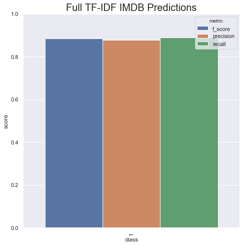
tf_idf.fit(x_train["review"], y_train)This model only takes a few seconds to train but gets a pretty decent F-score of .88 only using unigrams.
With this new model, we can find the most predictive features by simply grabbing the coefficient names from the TF-IDF Transformer and the coefficient values from our SVM.
coefs = tf_idf.named_steps["classifier"].coef_
if type(coefs) == csr_matrix:
    coefs.toarray().tolist()[0]
else:
    coefs.tolist()
feature_names = tf_idf.named_steps["tfidf"].get_feature_names()
coefs_and_features = list(zip(coefs[0], feature_names))
# Most positive features
sorted(coefs_and_features, key=lambda x: x[0], reverse=True)
# Most negative features
sorted(coefs_and_features, key=lambda x: x[0])
# Most predictive overall
sorted(coefs_and_features, key=lambda x: abs(x[0]), reverse=True)
We can grab the weights our model gives to each feature by accessing the “classifier” named step in our pipeline. When
creating a pipeline we name each step in the process so that we can access them with this named_steps function. Most
SciKit-Learn models have a .coef_ parameter which will return the coefficients of the model that we can use to find what
is most predictive. I do a little type checking around sparse matrices for convenience because these types of lexical
features can be very very sparse. The feature names are stored in the tfidf step of our pipeline we access it the same
way as the classifier but call the get_feature_names function instead.
Our top ten positive words are:
[(3.482397353551051, 'excellent'),
 (3.069350528649819, 'great'),
 (2.515865496104781, 'loved'),
 (2.470404287610431, 'best'),
 (2.4634974085860115, 'amazing'),
 (2.421134741115058, 'enjoyable'),
 (2.2237089115789166, 'perfect'),
 (2.196802503474607, 'fun'),
 (2.1811330282241426, 'today'),
 (2.1407707555282363, 'highly')]
and our top ten negative words are:
[(-5.115103657971178, 'worst'),
 (-4.486712890495122, 'awful'),
 (-3.676776745907702, 'terrible'),
 (-3.5051277582046536, 'bad'),
 (-3.4949920792779157, 'waste'),
 (-3.309000819824398, 'boring'),
 (-3.2772982524056973, 'poor'),
 (-2.9054813685114307, 'dull'),
 (-2.7129398526527253, 'nothing'),
 (-2.710497534821449, 'fails')]
Using our “Good” Features
Now that we’ve discovered some “good” features we can build even simpler models, or use these as features in other problems in a similar domain. Let’s build some simple rules that will return 1 if any of these predictive words are present in a review and 0 otherwise. Then retrain the model with only those 20 features and see how we do.
To do this I created a simple SciKit-Learn transformer which converts a list of n-grams to regex rules which NLTK’s tokenizer can search for. It’s not super fast (That’s an understatement it’s really slow. You should use the vocabulary parameter in the TfidfVectorizer instead, more to come.) but it’s easy to read and gets the job done.
from typing import List
from functools import reduce
import nltk
import pandas as pd
from sklearn.base import TransformerMixin, BaseEstimator

class RuleTransformer(TransformerMixin, BaseEstimator):

    def __init__(self, n_grams: List[List[str]]):
        self.n_grams = n_grams
        self.rules = [reduce(lambda x, y: x + r"<{}>".format(y), n_gram, "") for n_gram in n_grams]

    def transform(self, text: List[str]):
        if isinstance(text, pd.Series):
            text = text.tolist()

        featurized = []
        for sentence in text:
            tokenized = nltk.TokenSearcher(nltk.word_tokenize(sentence))

            features = []
            for rule in self.rules:
                features.append(1 if len(tokenized.findall(rule)) > 0 else 0)
            featurized.append(features)

        return featurized

    def get_feature_names(self):
        return self.n_grams

    def fit(self, X, y=None):
        """No fitting necessary so we just return ourselves"""
        return self
There are three main parts of this code.
Line 11 converts a tuple representing an n-gram so something like (“good”, “movie”) into a regex r”
Lines 13–26 perform the transformation by stopping through every sentence, or review in this case, in our input and applying each regex to that sentence. If the regex finds something it places a one in a list at the position corresponding to the n-gram that fired. This will produce a vector with 1’s and 0’s representing which n-grams are present in which sentences.
Lines 28–29 allow us to get the relevant feature names as we did before. It’s just convenient.
With this new handy-dandy transformer, we can retrain our model using just those top ten best, and bottom ten worst words.
n_grams = [('excellent',), ('great',), ('perfect',),
('best',), ('brilliant',), ('surprised',),
('hilarious',), ('loved',), ('today',),
('superb',), ('worst',), ('awful',),
('waste',), ('poor',), ('boring',),
('bad',), ('disappointment',), ('poorly',),
('horrible',), ('bored',)]
classifier = svm.LinearSVC(C=1.0, class_weight="balanced")
rules = Pipeline([
('rules', RuleTransformer(n_grams)),
("classifier", classifier)
])
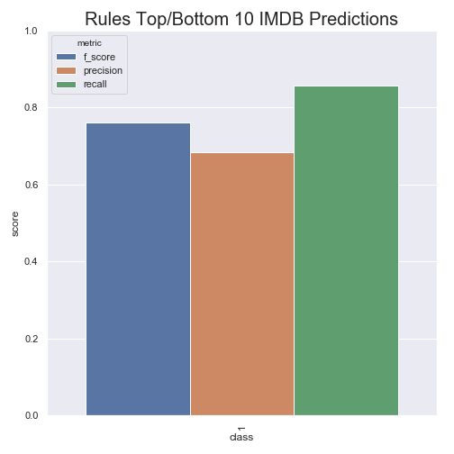
rules.fit(x_train["review"], y_train)These 20 features decrease our F1 by about .13 which may seem like a lot, but we are only using .03% of the original 65,247 words. That’s pretty neat! These 20 features encode a majority of the information in our data and we could use them as features in other pipelines!
TfidfVectorizer for Rule Extraction
I built that rule vectorizer above but we can get the same results by using the TfidfVectorizer and passing in a vocabulary parameter. The original SciKit-Learn vectorizer takes a parameter called vocabulary which accepts a dictionary mapping individual words, or n-grams separated by spaces, to integers. So to get the same effect we could have run:
top_feats = sorted(coefs_and_features,
                   key=lambda x: abs(x[0]),
                   reverse=True)[:20]
vocab = {x[1]: i for i, x in enumerate(top_feats)}
TfidfVectorizer(vocabulary=vocab)
Here we get the sorted list of features, then we create a map from feature name to integer index and pass it to the vectorizer. If you’re curious about what the map looks like it’s something like this:
{"great": 0,
 "poor": 1,
 "very poor": 2,
 "very poor performance": 3}
N-grams are represented by adding a space between the words. If we use the above code instead of our RuleTransformer we’ll get the same results in a fraction of the time.
How Many Features to Take?
Those 20 words seem to be pretty powerful. They can get us .79 F1 right out of the gate, but maybe 20 wasn’t the right number of features. We can find out by running our classifier on more and more of the top features and plotting the F1.
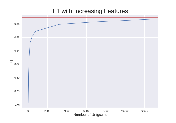
This shows us that the model starts to converge to the best TF-IDF unigram performance after about 13k of the most predictive words. So we can get the same performance with only 20% of our original feature set! Going forward using these 13k features is a more principled number and we still get a massive reduction in the number of original features.
Conclusion
If we are looking at purely lexical features, specific words, and their counts, then this can be a nice way of uncovering useful words and phrases. Language is much more complicated than simply the words you use. It’s important to look at all kinds of information when designing real systems. Use BERT, use syntactic features like how the sentence parses. There is so much more to language than just the raw words, but hopefully, this little trick can help you find some good words when you’re stuck.